Partition function (mathematics)

The partition function or configuration integral, as used in probability theory, information science and dynamical systems, is an abstraction of the definition of a partition function in statistical mechanics. It is a special case of a normalizing constant in probability theory, for the Boltzmann distribution. The partition function occurs in many problems of probability theory because, in situations where there is a natural symmetry, its associated probability measure, the Gibbs measure, has the Markov property. This means that the partition function occurs not only in physical systems with translation symmetry, but also in such varied settings as neural networks (the Hopfield network), and applications such as genomics, corpus linguistics and artificial intelligence, which employ Markov networks, and Markov logic networks. The Gibbs measure is also the unique measure that has the property of maximizing the entropy for a fixed expectation value of the energy; this underlies the appearance of the partition function in maximum entropy methods and the algorithms derived therefrom.

1 Definition
2 The parameter β
3 Symmetry
4 As a measure
5 Normalization
6 Expectation values
7 Correlation functions
8 General properties
9 See also

Definition

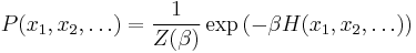
Given a set of random variables $X_i$ taking on values $x_i$ , and some sort of potential function or Hamiltonian $H(x_1,x_2,\dots)$ , the partition function is defined as

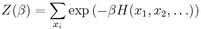
$Z(\beta) = \sum_{x_i} \exp \left(-\beta H(x_1,x_2,\dots) \right)$

The function H is understood to be a real-valued function on the space of states 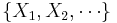$\{X_1,X_2,\cdots\}$ , while $\beta$ is a real-valued free parameter (conventionally, the inverse temperature). The sum over the $x_i$ is understood to be a sum over all possible values that the random variable $X_i$ may take. Thus, the sum is to be replaced by an integral when the $X_i$ are continuous, rather than discrete. Thus, one writes

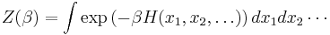
$Z(\beta) = \int \exp \left(-\beta H(x_1,x_2,\dots) \right) dx_1 dx_2 \cdots$

for the case of continuously-varying $X_i$ .

The number of variables $X_i$ need not be countable, in which case the sums are to be replaced by functional integrals. Although there are many notations for functional integrals, a common one would be

$Z = \int \mathcal{D} \phi \exp \left(- \beta H[\phi] \right)$

Such is the case for the partition function in quantum field theory.

A common, useful modification to the partition function is to introduce auxiliary functions. This allows, for example, the partition function to be used as a generating function for correlation functions. This is discussed in greater detail below.

The parameter β

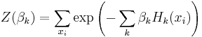
The role or meaning of the parameter $\beta$ is best understood by examining the derivation of the partition function with maximum entropy methods. Here, the parameter appears as a Lagrange multiplier; the multiplier is used to guarantee that the expectation value of some quantity is preserved by the distribution of probabilities. Thus, in physics problems, the use of just one parameter $\beta$ reflects the fact that there is only one expectation value that must be held constant: this is the energy. For the grand canonical ensemble, there are two Lagrange multipliers: one to hold the energy constant, and another (the fugacity) to hold the particle count constant. In the general case, there are a set of parameters taking the place of $\beta$ , one for each constraint enforced by the multiplier. Thus, for the general case, one has

$Z(\beta_k) = \sum_{x_i} \exp \left(-\sum_k\beta_k H_k(x_i) \right)$

The corresponding Gibbs measure then provides a probability distribution such that the expectation value of each $H_k$ is a fixed value.

Although the value of $\beta$ is commonly taken to be real, it need not be, in general; this is discussed in the section Normalization below.

Symmetry

The potential function itself commonly takes the form of a sum:

$H(x_1,x_2,\dots) = \sum_s E(s)\,$

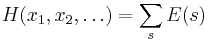
where the sum over s is a sum over some subset of the power set P(X) of the set $X=\lbrace x_1,x_2,\dots \rbrace$ . For example, in statistical mechanics, such as the Ising model, the sum is over pairs of nearest neighbors. In probability theory, such as Markov networks, the sum might be over the cliques of a graph; so, for the Ising model and other lattice models, the maximal cliques are edges.

The fact that the potential function can be written as a sum usually reflects the fact that it is invariant under the action of a group symmetry, such as translational invariance. Such symmetries can be discrete or continuous; they materialize in the correlation functions for the random variables (discussed below). Thus a symmetry in the Hamiltonian becomes a symmetry of the correlation function (and vice-versa).

This symmetry has a critically important interpretation in probability theory: it implies that the Gibbs measure has the Markov property; that is, it is independent of the random variables in a certain way, or, equivalently, the measure is identical on the equivalence classes of the symmetry. This leads to the widespread appearance of the partition function in problems with the Markov property, such as Hopfield networks.

As a measure

The value of the expression

$\exp \left(-\beta H(x_1,x_2,\dots) \right)$

can be interpreted as a likelihood that a specific configuration of values $(x_1,x_2,\dots)$ occurs in the system. Thus, given a specific configuration $(x_1,x_2,\dots)$ ,

$P(x_1,x_2,\dots) = \frac{1}{Z(\beta)} \exp \left(-\beta H(x_1,x_2,\dots) \right)$

is the probability of the configuration $(x_1,x_2,\dots)$ occurring in the system, which is now properly normalized so that 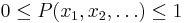$0\le P(x_1,x_2,\dots)\le 1$ , and such that the sum over all configurations totals to one. As such, the partition function can be understood to provide a measure on the space of states; it is sometimes called the Gibbs measure. More narrowly, it is called the canonical ensemble in statistical mechanics.

There exists at least one configuration $(x_1,x_2,\dots)$ for which the probability is maximized; this configuration is conventionally called the ground state. If the configuration is unique, the ground state is said to be non-degenerate, and the system is said to be ergodic; otherwise the ground state is degenerate. The ground state may or may not commute with the generators of the symmetry; if commutes, it is said to be an invariant measure. When it does not commute, the symmetry is said to be spontaneously broken.

Conditions under which a ground state exists and is unique are given by the Karush–Kuhn–Tucker conditions; these conditions are commonly used to justify the use of the Gibbs measure in maximum-entropy problems.

Normalization

The values taken by $\beta$ depend on the mathematical space over which the random field varies. Thus, real-valued random fields take values on a simplex: this the geometrical way of saying that the sum of probabilities must total to one. For quantum mechanics, the random variables ranges over complex projective space (or complex-valued Hilbert space), because the random variables are interpreted as probability amplitudes. The emphasis here is on the word projective, as the amplitudes are still normalized to one. The normalization for the potential function is the Jacobian for the appropriate mathematical space: it is 1 for ordinary probabilities, and i for complex Hilbert space; thus, in quantum field theory, one sees $it H$ in the exponential, rather than $\beta H$ .

Expectation values

The partition function is commonly used as a generating function for expectation values of various functions of the random variables. So, for example, taking $\beta$ as an adjustable parameter, then the derivative of $\log(Z(\beta))$ with respect to $\beta$

$\bold{E}[H] = \langle H \rangle = -\frac {\partial \log(Z(\beta))} {\partial \beta}$

gives the average (expectation value) of H. In physics, this would be called the average energy of the system.

The entropy is given by

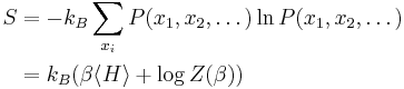
$\begin{align} S & = -k_B\sum_{x_i} P(x_1,x_2,\dots) \ln P(x_1,x_2,\dots) \\ & = k_B(\beta \langle H\rangle %2B \log Z(\beta)) \end{align}$

The Gibbs measure is the unique statistical distribution that maximizes the entropy for a fixed expectation value of the energy; this underlies its use in maximum entropy methods.

By introducing artificial auxiliary functions $J_k$ into the partition function, it can then be used to obtain the expectation value of the random variables. Thus, for example, by writing

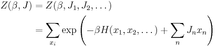
$\begin{align} Z(\beta,J) & = Z(\beta,J_1,J_2,\dots) \\ & = \sum_{x_i} \exp \left(-\beta H(x_1,x_2,\dots) %2B \sum_n J_n x_n \right) \end{align}$

one then has

$\bold{E}[x_k] = \langle x_k \rangle = \left. \frac{\partial}{\partial J_k} \log Z(\beta,J)\right|_{J=0}$

as the expectation value of $x_k$ .

Correlation functions

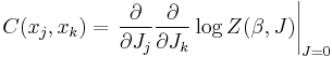
Multiple differentiations lead to the correlation functions of the random variables. Thus the correlation function $C(x_j,x_k)$ between variables $x_j$ and $x_k$ is given by:

$C(x_j,x_k) = \left. \frac{\partial}{\partial J_j} \frac{\partial}{\partial J_k} \log Z(\beta,J)\right|_{J=0}$

For the case where H can be written as a quadratic form involving a differential operator, that is, as

$H = \frac{1}{2} \sum_n x_n D x_n$

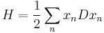
then the correlation function $C(x_j,x_k)$ can be understood to be the Green's function for the differential operator (and generally giving rise to Fredholm theory).

General properties

Partition functions often show critical scaling, universality and are subject to the renormalization group.